Level curves; partial derivatives; tangent plane approximation
Table of Contents
The course, to ensure simplicity, focuses on functions of 2 and 3 variables, but everything discussed in my notes is applicable to functions of more variables as well.
From geometry to functions of several functions.
Introducing multivariable functions
Think of a random ordinary function of one variable, such as:
\begin{equation} f(x) = \sin{x} \end{equation}
We have an easy way of dealing with these functions and that is by plotting them
in the form of \(y = f(x)\):

This can not be used, as is, for functions of more variables. It needs a slight modification, since these functions would not normally be properly plotted on the plane.
Let’s now see what a function of two variables looks like:
\begin{equation} f:\mathbb{R}^2\to \mathbb{R}: (x,y)\to f(x,y) \end{equation}It is just like any other function we already know (It has a domain of definition, certain sets of input for which it may not be defined)!
Some examples of such functions are:
\begin{align*} f(x,y)&=x^2+y^2\\ f(x,y)&=\sqrt{y}\\ f(x,y)&= \frac{1}{x+y} \end{align*}Visualizing functions
Truth be told, while functions with two variables are slightly more difficult than our common functions in visualization, they can be easily perceived. That changes when we talk about functions of more variables making it increasingly more difficult for us to visualize them.1
Just like we got used to seeing \(y=f(x)\), it is easy, especially if you sit in front of a computer, to plot a function of two variables by using: \(z=f(x,y)\).
Some examples of such plots:
- \(f(x,y)=-y\)

- \(f(x,y) = 1-x^2-y^2\)

- \(f(x,y)=y^2-x^2\)
 The first time we see a saddle point, in which we will be interested in
the near future.
The first time we see a saddle point, in which we will be interested in
the near future.
Understanding a three-dimensional plot
It is not necessary however, to use a computer to generate such a plot. Obviously, it will make our lives significantly easier and will ensure a good result, one that will be presentable and clear to others as well, but it is not needed.
Even though it gets increasingly more tiring for more complex functions a good approach to designing the three dimensional plot of a given function \(f\), is taking the common points that it has with different planes ( such as the \(xy,xz,yz\) planes )2
Contour plots:
So far, following the simple path, we built upon what we already knew and managed to describe every function of two variables in the three dimensional space. Now let’s take a step back.
Think of the difficulty which drawing 3d plots presents. We can not reliably represent complex 3d shapes on paper. Most of the times it will be extremely difficult for the reader to understand what exactly we’re plotting. That’s where contour plots come in. They are a collection of curves in the form of \(f(x,y) = c\in \mathbb{R}\).
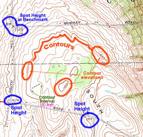
An easy way to understand what contour plots are is by looking at an ordinary map ( such as the one below ), and look how height is embedded in it. Interesting is not it3?
Octave code for simple contour plots:
[x,y] = meshgrid(-10:0.1:10,-10:01.:10)
contour(x.^2+y.^2)
That ( with the slight change of using the contourf instead of the contour
func ) gives us:

Contour plots applications
Just like we have already seen, contour plots are often met in mapsThere are many applications in maps, being able to get information on the location generally:
- Heat maps
- Height maps
- Population maps
Examples
Linking to the previous examples, their contour plots:
- \(f(x,y) = -y\)

- \(f(x,y)= 1-x^2-y^2\)

- \(f(x,y)=x^2-y^2\)

Partial Derivatives
Now think of a random contour plot. Just by looking at it we can understand in just one look how moving on the plane is going to affect our function’s values. More specifically, we can see that if we move on a contour plot, our function’s value will remain constant, while in any other case it will increase or decrease. We can also see ( if we are careful enough ) in which direction the function increases at a maximum rate.
Thus, we can intuitively understand the rate of change, which we know as the derivative of a function:
Remember
For a function of one variable the derivative is given as:
\begin{equation} f'(x) = \frac{d{f}}{d{x}} = \lim_{\Delta{x}\to 0 }\frac{f(x+\Delta f(x)}{\Delta x} \end{equation}Differentiability
Obviously, we can not compute the derivative of each and every function. There are some functions for which the derivative does not exist and that remains true for functions of more variables. It is good to remember it, yet outside the scope of this course.
Approximation formula
If we know the value of \(f,f'\) at a point \(x_0\) we can approximate the value of \(f\) at \(x\), provided that \(x\) is close to \(x_0\) using the following formula:
\begin{equation} f(x)\approx f(x_0) + f'(x_0)(x-x_0) \end{equation}What changes
The difficulty presented in functions of more variables is that we can change more than one variable and we can also change both of them in UNLIMITED combinations.
We, then, create a new form of a derivative, the partial derivative, which shows us how \(f\) would change should we modify only a specific parameter, such as \(x\) or \(y\):
\begin{equation} \frac{\partial{f}}{\partial{x}} = \lim_{\Delta x \to 0} \frac{f(x_0+\Delta x,y_0)-f(x_0,y_0)}{\Delta x} \end{equation}Geometric implications
It is interesting noting down that partial derivatives can be easily found in 3d plots as well. Let’s pick one of the previous 3d plots and focus on calculating the partial derivative \(\frac{\partial{f}}{\partial{x}}\). To do that we only need to follow this algorithm:
- Given a 3d plot of our function
- Draw a plane in the form of \(y = y_{0}\in \mathbb{R}\)
- Focus on their intersection
- Think of the plane of step 2 as a two dimensional plane and the points where it intersects \(f\) as the plot of a single variable function \(g\)
- In this two-dimensional graph we see that \(y = g(x)\)
- For every \(x\in D_g \subset \mathbb{R}\) it is true that \(\frac{d{g}}{d{x}} = \frac{\partial{f}}{\partial{x}} (x,y_0)\)
Computing partial derivatives
Just like normal derivatives we won’t rely on limits to compute them. The rules we know are applicable to partial derivatives as well, we just need to slightly change them for a multi-dimensional space.
Using what we already know we can compute a partial derivative by considering every other variable as a constant. An example follows:
\begin{align*} f(x,y) &= x + y\\ \frac{\partial{f}}{\partial{x}} &= \frac{\partial{(x+y)}}{\partial{x}} = \frac{d{x+c}}{d{x}} = 1 \end{align*}Footnotes:
Of course, one could argue that with the help of computers we could implement a plotting solution for functions with 3 variables by including the time factor there. It certainly seems like a good idea to try.
Afterall, this is how the computer draws the graphs. We may not have the raw computational power but… we know the algorithm
Think of it like that: \(height = f(x,y)\), which essentially translates that every contour plot on the map shows a level of constant height: \(height = c \in \mathbb{R}\)